PREVIOUS YEAR SOLVED PAPERS - July 2018
21. In a perfectly competitive market, a firm in the long run operates at the level of output where:


- Option : D
- Explanation : In the case of perfect competition, average revenue, AR being equal to the selling price, must be identical to MR curve for the same reason that the firm cannot influence price level. Now the unit profit level for the firm is given by AR = Min. AC.
The long-run equilibrium of the firm is now complete. Optimal output level is determined by equating MR = MC, in which case, the individual entrepreneur has no incentive to alter the optimal level of output.
Long-run ‘normal profits’ are now earned at, p = Min. AC, in which case there is no incentive for a firm to enter or leave the industry to which the firm belongs.
The concept of competition influencing price and output determination needs to be pointed out. If p > MC, then π > 0. This would induce other firms to enter the industry. Consequently, the total supply of output to the industry by all such firms will increase. Consequently, supply p will be driven down. On the other hand, if p < MC, then π < 0. Now firms will start to leave the industry. The supply of total output will decline. This will drive up price. Finally, with movements from both below and above MC values, the final value of price will be where, p = MC.
Because supply prices of output of a perfectly competitive firm are set in this way along the rising portion of the MC curve, this turns out to be the supply curve of the firm’s output.
Finally, with all the above results in the situation where the firm is a price-taker in perfect competition, we obtain the compressed result for pricing of output of a firm in perfectly competitive market:
p = MC = Min. AC = AR = MR
Such a firm is the most efficient one in terms of its minimum average cost of production, maximal output that earns the firm the full range of economies of scale, and maximal profits at this level that shows that the entire output is fully distributed among factors of production.
22. Assignment of numerals to the objects to represent their attributes is known as:
- Option : A
- Explanation : Nominal Scale: When data are labels or names used to identify the attribute of an element, then the nominal scale is used. For example, assume that a marketing research company wants to conduct a survey in three towns of India—Bhopal, Nagpur and Baroda. While compiling the data, the company assigns the numeric code “1” to Bhopal, “2” to Nagpur, and “3” to Baroda. In this case, “1”, “2”, and “3” are the labels used to identify the three different towns. Data shows the numeric value but the scale of measurement is nominal. In other words, we cannot say that “1” indicates any ranking or any rating, this is only for the sake of convenience in identification. Employee identification numbers, contributory provident fund numbers, personal identification number (PAN), and the like are some other examples of nominal data. Nominal level measurement is the lowest level of data measurement.
Ordinal Scale: In addition to nominal level data capacities, the ordinal scale can be used to rank or order objects. For example, a manufacturing company administers a questionnaire to 150 consumers for obtaining the consumer perception for one of its products. Each consumer is asked to judge between three given options, excellent, good, or poor. Clearly, excellent is ranked the best and poor the worst with good ranked between the two. If we want to assign numeric values to these three attributes, “1” can be used for excellent, “2” for good, and “3” for poor. In most cases, when we apply statistical tools and techniques, for the sake of interpretation convenience, rankings are set in reverse. In this case, “1” will be used for poor, “2” for good, and “3” for excellent. Therefore, the lowest number has the lowest ranking, and the highest number has the highest ranking. While using this kind of ordinal measurement, the company cannot say that the interval between ranking points 1 and 2 is equal to the interval between ranking points 2 and 3. Here, it can be stated that 1 is superior followed by 2 and 3, or as in the second case 1, the lowest number, has got the lowest ranking followed by the next two numbers, 2 and 3, as the ranking reference for good and excellent. The exact difference between these numeric values cannot be measured in any of these cases. Nominal and ordinal level data measurement are often used for imprecise measurements such as demographic questions, ranking of items under the study, and the like. This is why these data are termed as nonmetric data and are referred to as qualitative data.
Interval Scale: In the interval level measurement, the difference between two consecutive numbers is meaningful. Interval data is always numeric. For example, three students of MSc Statistics have scored 65, 75, and 85 in the subject reliability theory. These three students can be rated in terms of their performances. However, the difference in the numbers is also meaningful. The student who secured 85 marks is the highest ranking performer whereas the student who secured 65 is the lowest with the student who secured 75 marks in the middle. In interval level measurement, meaningful difference between two ranking points can be obtained. In the above example, we can also compute that between the highest and the lowest ranking points, the difference is 20 marks.
Ratio Scale: Ratio level measurements possess all the properties of interval data with meaningful ratio of two values. The ratio scale must contain a zero value that indicates that nothing exists for the variable at zero point. For example, a company markets two toothbrushes priced Rs.30 and Rs.15, respectively. In the ratio scale, the difference between the two prices, that is, Rs.30 – Rs.15 = Rs.15, can be calculated and is meaningful. With it, we can also say that the price of the first product Rs.30 is two times that of the second product priced at Rs.15. Interval and ratio level data are collected using some precise instruments. These data are called metric data and are sometimes referred to as quantitative data.
23. A graph of a cumulative frequency distribution is called:
- Option : C
- Explanation : A graph is a geometrical image of frequency distribution. It is a mathematical picture. Frequency distributions are converted into visual models to facilitate understanding. It is easier, more convenient and quicker to draw inferences from graphs than from frequency distribution. Comparison of data also becomes easier. Graphical representation in the form of histogram, frequency polygons, cumulative frequency curves (ogive), Pie graphs etc., appear almost daily in the newspapers, magazines, trade publications, business reports and scientific periodicals.
- Option : C
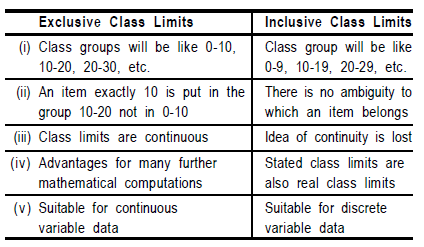
- Explanation : If the upper limit of a class is excluded from the interval, it is exclusive method of classification, otherwise it is inclusive method of classification.
Distinguish between Open End Classes and Close End Classes
When lower limit of first class interval and upper limit of last intervals are not given, these are called open end classes and when these limits are given, these are called close end classes.
25. For a standard normal probability distribution, the mean (μ) and the standard deviation (σ) are:
- Option : A
- Explanation : Standard Normal Probability Distribution: To deal with problems where the normal probability distribution is applicable, the value of random variable x is standardized by expressing it as the number of standard deviations (σ) lying on both sides of its mean (μ). Such standardized normal random variable, z (also called z-statistic, z-score or normal variable) is defined as:

or equivalently
The z-statistic measures the number of standard deviations that any value of the random variable x falls from the mean. From formula, we may conclude that
(i) When x is less than the mean (μ), the value of z is negative.
(ii) When x is more than the mean (μ), the value of z is positive.
(iii) When x = μ, the value of z = 0.
Standard Normal Probability Distribution:
A normal probability distribution with mean equal to zero and standard deviation equal to one.
